6 Scaling

In this chapter we’ll mostly compare Polars to Dask rather than to Pandas. This isn’t an apples-to-apples comparison, because Dask helps scale Pandas but it might help scale Polars too one day. Dask, like Spark, can run on a single node or on a cluster with thousands of nodes.

Polars launched its cloud offering in September 2025 with support for AWS, with on-premises support announced in June 2026. However, at the time of writing, these are not free offerings, and open source Polars is still single-node only.

Polars does have a streaming mode for larger-than-memory datasets on a single machine. It also uses memory more efficiently than Pandas. These two things mean you can use Polars for much bigger data than Pandas can handle, and hopefully you won’t need tools like Dask or Spark until you’re actually running on a cluster.

Note

I use “Dask” here as a shorthand for dask.dataframe. Dask does a bunch of other stuff too.

Warning

In older versions of Polars, streaming mode was enabled by passing streaming=True to collect, but in newer versions you should pass engine="streaming". The old way still works but is deprecated and will be removed in a future version.

6.1 Get the data

We’ll be using political donation data from the FEC. Warning: this takes a few minutes.

import asyncio
from zipfile import ZipFile
from pathlib import Path
from datetime import date
from io import BytesIO
import httpx
import polars as pl
import pandas as pd


pl.Config.set_tbl_rows(5)
pd.options.display.max_rows = 5

fec_dir = Path("../data/fec")

async def download_and_save_cm(year: str, client: httpx.AsyncClient):
    cm_cols = ["CMTE_ID", "CMTE_NM", "CMTE_PTY_AFFILIATION"]
    dtypes = {"CMTE_PTY_AFFILIATION": pl.Categorical}
    url = f"https://www.fec.gov/files/bulk-downloads/20{year}/cm{year}.zip"
    resp = await client.get(url)
    with ZipFile(BytesIO(resp.content)) as z:
        pl.read_csv(
            z.read("cm.txt"),
            has_header=False,
            columns=[0, 1, 10],
            new_columns=cm_cols,
            separator="|",
            schema_overrides=dtypes,
        ).write_parquet(fec_dir / f"cm{year}.pq")

async def download_and_save_indiv(year: str, client: httpx.AsyncClient):
    dtypes = {
        "CMTE_ID": pl.String,
        "EMPLOYER": pl.Categorical,
        "OCCUPATION": pl.Categorical,
        "TRANSACTION_DT": pl.String,
        "TRANSACTION_AMT": pl.Int32,
    }
    url = f"https://www.fec.gov/files/bulk-downloads/20{year}/indiv{year}.zip"
    resp = await client.get(url)
    with ZipFile(BytesIO(resp.content)) as z:
        pl.read_csv(
            z.read("itcont.txt"),
            has_header=False,
            columns=[0, 11, 12, 13, 14],
            new_columns=list(dtypes.keys()),
            separator="|",
            schema_overrides=dtypes,
            encoding="cp1252",
        ).with_columns(
            pl.col("TRANSACTION_DT").str.to_date(format="%m%d%Y", strict=False)
        ).write_parquet(
            fec_dir / f"indiv{year}.pq"
        )

years = ["08", "10", "12", "14", "16"]
if not fec_dir.exists():
    fec_dir.mkdir()
    async with httpx.AsyncClient(follow_redirects=True, timeout=None) as client:
        cm_tasks = [download_and_save_cm(year, client) for year in years]
        indiv_tasks = [download_and_save_indiv(year, client) for year in years]
        tasks = cm_tasks + indiv_tasks
        await asyncio.gather(*tasks)

6.2 Simple aggregation

Suppose we want to find the most common occupations among political donors. Let’s assume that this data is too big for your machine’s memory to read it in all at once.

We can solve this using Polars streaming, using Dask’s lazy dataframe or simply using Pandas to read the files one by one and keeping a running total:

occupation_counts_pl = (
    pl.scan_parquet(fec_dir / "indiv*.pq", cache=False)
    .select(pl.col("OCCUPATION").value_counts(parallel=True, sort=True))
    .collect(engine="streaming")
)
occupation_counts_pl

shape: (579_159, 1)

OCCUPATION
struct[2]
{"RETIRED",4773715}
{"NOT EMPLOYED",2715939}
{null,1439867}
…
{"PROFESSOR OF PYSICS",1}
{"ARTIST/SINGER-SONGWRITER",1}

import dask.dataframe as dd
from dask import compute
occupation_counts_dd = dd.read_parquet(
    fec_dir / "indiv*.pq", engine="pyarrow", columns=["OCCUPATION"]
)["OCCUPATION"].value_counts()
occupation_counts_dd.compute()

OCCUPATION
RETIRED                     4773715
NOT EMPLOYED                2715939
                             ...   
PROFESSOR OF PYSICS               1
ARTIST/SINGER-SONGWRITER          1
Name: count, Length: 579158, dtype: int64

files = sorted(fec_dir.glob("indiv*.pq"))

total_counts_pd = pd.Series(dtype="int64")

for year in files:
    occ_pd = pd.read_parquet(year, columns=["OCCUPATION"], engine="pyarrow")
    counts = occ_pd["OCCUPATION"].value_counts()
    total_counts_pd = total_counts_pd.add(counts, fill_value=0).astype("int64")

total_counts_pd.nlargest(100)

OCCUPATION
RETIRED         4773715
NOT EMPLOYED    2715939
                 ...   
SURGEON           25545
OPERATOR          25161
Length: 100, dtype: int64

Note

Polars can handle some larger-than-memory data even without streaming. Thanks to predicate pushdown, we can filter dataframes without reading all the data into memory first. So streaming mode is most useful for cases where we really do need to read in a lot of data.

6.3 Executing multiple queries in parallel

Often we want to generate multiple insights from the same data, and we need them in separate dataframes. In this case, using collect_all is more efficient than calling .collect multiple times, because Polars can avoid repeating common operations like reading the data.

Let’s compute the average donation size, the total donated by employer and the average donation by occupation:

%%time
indiv_pl = pl.scan_parquet(fec_dir / "indiv*.pq")
avg_transaction_lazy_pl = indiv_pl.select(pl.col("TRANSACTION_AMT").mean())
total_by_employer_lazy_pl = (
    indiv_pl.drop_nulls("EMPLOYER")
    .group_by("EMPLOYER")
    .agg([pl.col("TRANSACTION_AMT").sum()])
    .sort("TRANSACTION_AMT", descending=True)
    .head(10)
)
avg_by_occupation_lazy_pl = (
    indiv_pl.group_by("OCCUPATION")
    .agg([pl.col("TRANSACTION_AMT").mean()])
    .sort("TRANSACTION_AMT", descending=True)
    .head(10)
)

avg_transaction_pl, total_by_employer_pl, avg_by_occupation_pl = pl.collect_all(
    [avg_transaction_lazy_pl, total_by_employer_lazy_pl, avg_by_occupation_lazy_pl],
    engine="streaming",
)

CPU times: user 21 s, sys: 527 ms, total: 21.5 s
Wall time: 866 ms

%%time
indiv_dd = (
    dd.read_parquet(fec_dir / "indiv*.pq", engine="pyarrow")
    # pandas and dask want datetimes but this is a date col
    .assign(
        TRANSACTION_DT=lambda df: dd.to_datetime(df["TRANSACTION_DT"], errors="coerce")
    )
)
avg_transaction_lazy_dd = indiv_dd["TRANSACTION_AMT"].mean()
total_by_employer_lazy_dd = (
    indiv_dd.groupby("EMPLOYER", observed=True)["TRANSACTION_AMT"].sum().nlargest(10)
)
avg_by_occupation_lazy_dd = (
    indiv_dd.groupby("OCCUPATION", observed=True)["TRANSACTION_AMT"].mean().nlargest(10)
)
avg_transaction_dd, total_by_employer_dd, avg_by_occupation_dd = compute(
    avg_transaction_lazy_dd, total_by_employer_lazy_dd, avg_by_occupation_lazy_dd
)

CPU times: user 9.56 s, sys: 2.3 s, total: 11.9 s
Wall time: 8.42 s

The Polars code above tends to be ~10x faster than Dask on my machine.

We should also profile memory usage, since it could be the case that Polars is just running faster because it’s reading in bigger chunks. According to the memray profiler, the Dask example’s memory usage peaks at ~4.0 GB, while Polars peaks at ~1.6 GB, so Polars wins on memory too.

Before I forget, here are the results of our computations:

6.3.1 avg_transaction

avg_transaction_pl

shape: (1, 1)

TRANSACTION_AMT
f64
563.97184

avg_transaction_dd

np.float64(563.9718398183915)

6.3.2 total_by_employer

total_by_employer_pl

shape: (10, 2)

EMPLOYER	TRANSACTION_AMT
cat	i32
"RETIRED"	1023306104
"SELF-EMPLOYED"	834757599
"N/A"	688186834
…	…
"FAHR, LLC"	166679844
"CANDIDATE"	75187243

total_by_employer_dd

EMPLOYER
RETIRED          1023306104
SELF-EMPLOYED     834757599
                    ...    
FAHR, LLC         166679844
CANDIDATE          75187243
Name: TRANSACTION_AMT, Length: 10, dtype: int32

6.3.3 avg_by_occupation

avg_by_occupation_pl

shape: (10, 2)

OCCUPATION	TRANSACTION_AMT
cat	f64
"CHAIRMAN CEO & FOUNDER"	1.0233e6
"PAULSON AND CO., INC."	1e6
"CO-FOUNDING DIRECTOR"	875000.0
…	…
"OWNER, FOUNDER AND CEO"	500000.0
"PERRY HOMES"	500000.0

avg_by_occupation_dd

OCCUPATION
CHAIRMAN CEO & FOUNDER              1.023333e+06
PAULSON AND CO., INC.               1.000000e+06
                                        ...     
OWNER, FOUNDER AND CEO              5.000000e+05
CHIEF EXECUTIVE OFFICER/PRODUCER    5.000000e+05
Name: TRANSACTION_AMT, Length: 10, dtype: float64

6.4 Filtering

Let’s filter for only the 10 most common occupations and compute some summary statistics:

6.4.1 avg_by_occupation, filtered

Getting the most common occupations:

top_occupations_pl = (
    occupation_counts_pl.select(
        pl.col("OCCUPATION")
        .struct.field("OCCUPATION")
        .drop_nulls()
        .head(10)
    )
    .to_series()
)
top_occupations_pl

shape: (10,)

OCCUPATION
cat
"RETIRED"
"NOT EMPLOYED"
"ATTORNEY"
…
"EXECUTIVE"
"ENGINEER"

top_occupations_dd = occupation_counts_dd.head(10).index
top_occupations_dd

CategoricalIndex(['RETIRED', 'NOT EMPLOYED', 'ATTORNEY', 'PHYSICIAN',
                  'HOMEMAKER', 'PRESIDENT', 'PROFESSOR', 'CONSULTANT',
                  'EXECUTIVE', 'ENGINEER'],
                 categories=['PUBLIC RELATIONS CONSULTANT', 'PRESIDENT', 'PHYSICIAN', 'SENIOR EXECUTIVE', ..., 'SR DIRECTOR, PRODUCT', 'PROFESSOR OF PYSICS', 'ARTIST/SINGER-SONGWRITER', 'SPECIAL PROJECTS MEDICAL CODER'], ordered=False, dtype='category', name='OCCUPATION')

donations_pl_lazy = (
    indiv_pl.filter(pl.col("OCCUPATION").is_in(top_occupations_pl.to_list()))
    .group_by("OCCUPATION")
    .agg(pl.col("TRANSACTION_AMT").mean())
)
total_avg_pl, occupation_avg_pl = pl.collect_all(
    [indiv_pl.select(pl.col("TRANSACTION_AMT").mean()), donations_pl_lazy],
    engine="streaming",
)

donations_dd_lazy = (
    indiv_dd[indiv_dd["OCCUPATION"].isin(top_occupations_dd)]
    .groupby("OCCUPATION", observed=True)["TRANSACTION_AMT"]
    .mean()
    .dropna()
)
total_avg_dd, occupation_avg_dd = compute(
    indiv_dd["TRANSACTION_AMT"].mean(), donations_dd_lazy
)

6.4.2 Plotting

These results are small enough to plot:

ax = (
    occupation_avg_pl
    .to_pandas()
    .set_index("OCCUPATION")
    .squeeze()
    .sort_values(ascending=False)
    .plot.barh(color="k", width=0.9)
)
lim = ax.get_ylim()
ax.vlines(total_avg_pl, *lim, color="C1", linewidth=3)
ax.legend(["Average donation"])
ax.set(xlabel="Donation Amount", title="Average Donation by Occupation")

[Text(0.5, 0, 'Donation Amount'),
 Text(0.5, 1.0, 'Average Donation by Occupation')]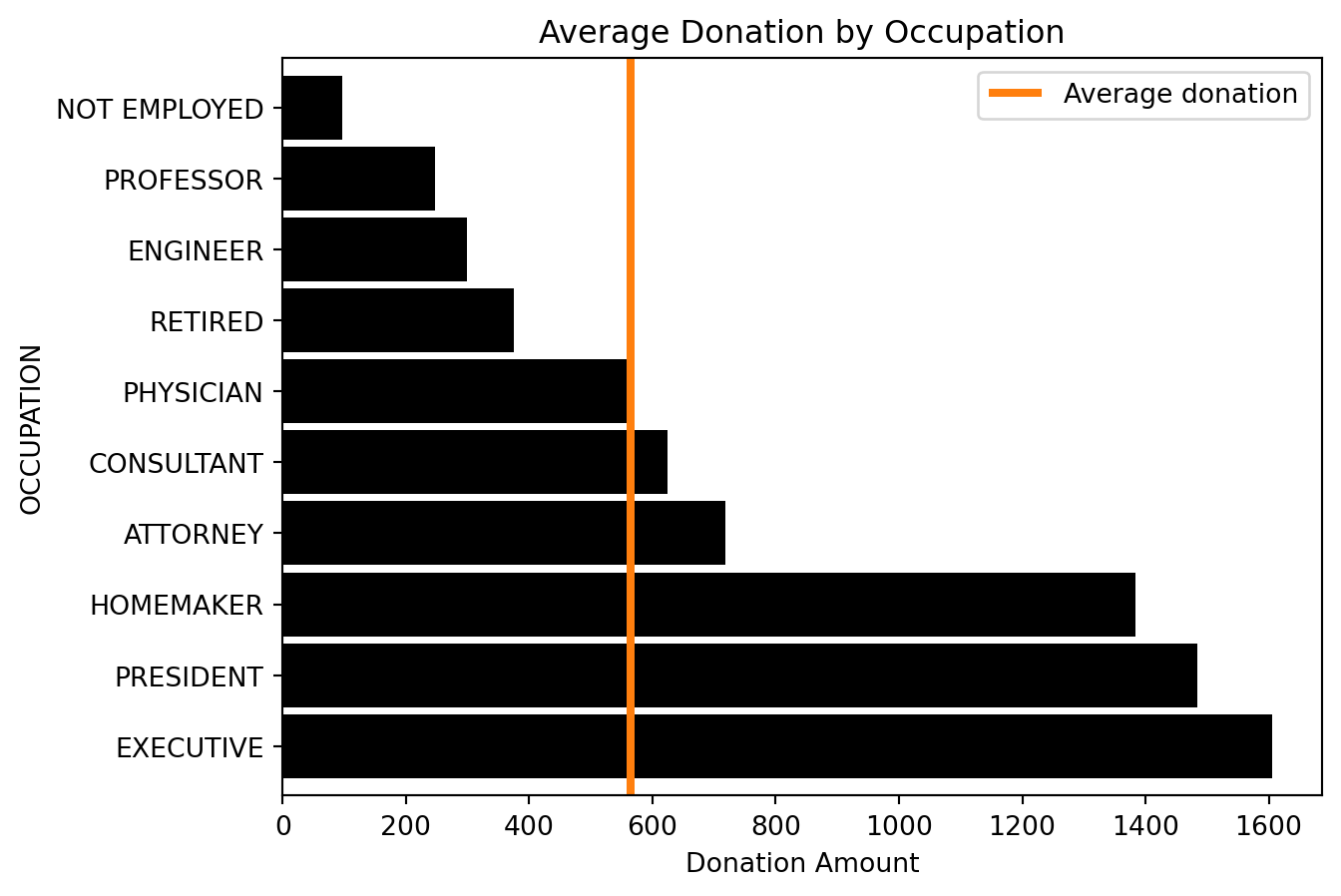

ax = occupation_avg_dd.sort_values(ascending=False).plot.barh(color="k", width=0.9)
lim = ax.get_ylim()
ax.vlines(total_avg_dd, *lim, color="C1", linewidth=3)
ax.legend(["Average donation"])
ax.set(xlabel="Donation Amount", title="Average Donation by Occupation")

[Text(0.5, 0, 'Donation Amount'),
 Text(0.5, 1.0, 'Average Donation by Occupation')]

6.5 Resampling

Resampling is another useful way to get our data down to a manageable size:

daily_pl = (
    indiv_pl.select(["TRANSACTION_DT", "TRANSACTION_AMT"])
    .drop_nulls()
    .sort("TRANSACTION_DT")
    .group_by_dynamic("TRANSACTION_DT", every="1d")
    .agg(pl.col("TRANSACTION_AMT").sum())
    .filter(
        pl.col("TRANSACTION_DT")
        .is_between(date(2011, 1, 1), date(2017, 1, 1), closed="left")
    )
    .with_columns(pl.col("TRANSACTION_AMT") / 1000)
    .collect(engine="streaming")
)
ax = (
    daily_pl.select(
        [pl.col("TRANSACTION_DT").cast(pl.Datetime), "TRANSACTION_AMT"]
    )
    .to_pandas()
    .set_index("TRANSACTION_DT")
    .squeeze()
    .plot(figsize=(12, 6))
)
ax.set(ylim=0, title="Daily Donations", ylabel="$ (thousands)")

[(0.0, 83407.5242),
 Text(0.5, 1.0, 'Daily Donations'),
 Text(0, 0.5, '$ (thousands)')]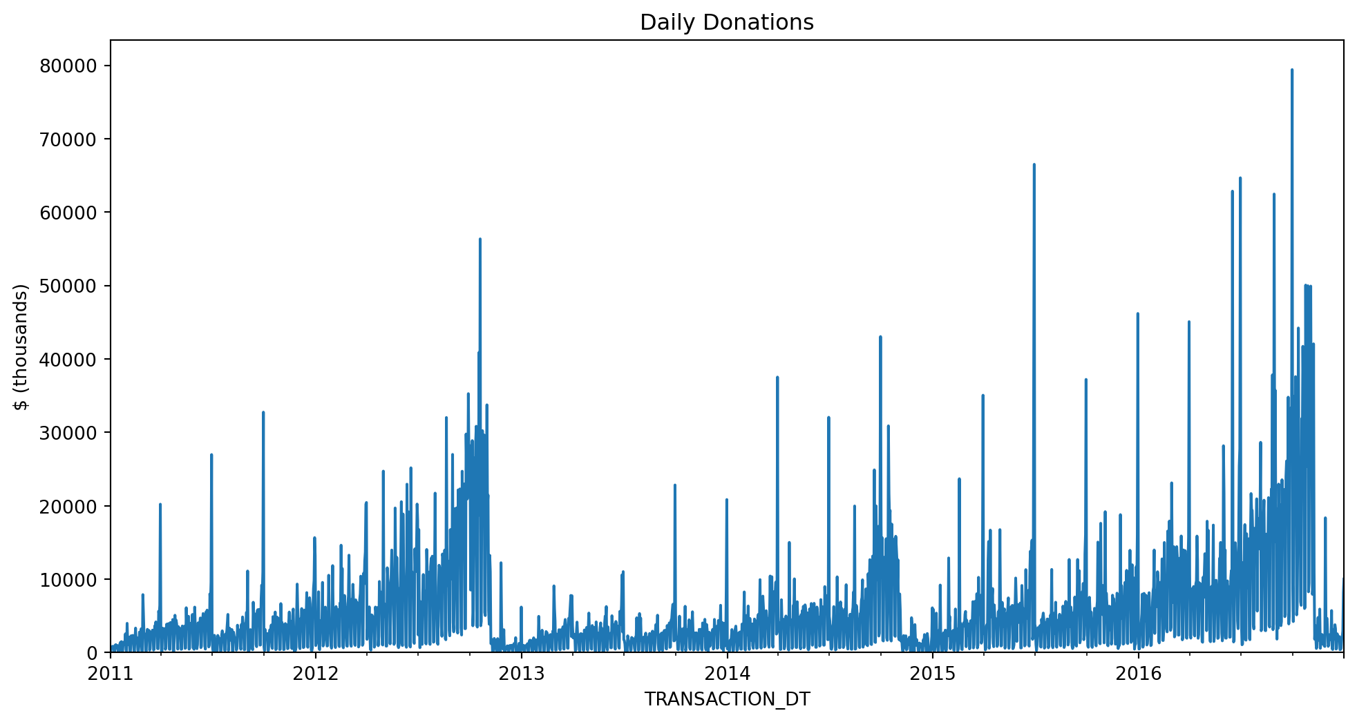

daily_dd = (
    indiv_dd[["TRANSACTION_DT", "TRANSACTION_AMT"]]
    .dropna()
    .set_index("TRANSACTION_DT")["TRANSACTION_AMT"]
    .resample("D")
    .sum()
    .loc["2011":"2016"]
    .div(1000)
    .compute()
)

ax = daily_dd.plot(figsize=(12, 6))
ax.set(ylim=0, title="Daily Donations", ylabel="$ (thousands)")

[(0.0, 83407.5242),
 Text(0.5, 1.0, 'Daily Donations'),
 Text(0, 0.5, '$ (thousands)')]

6.6 Joining

Polars joins work in streaming mode. Let’s add join the donations data with the committee master data, which contains information about the committees people donate to.

cm_pl = (
    pl.scan_parquet(fec_dir / "cm*.pq")
    # Some committees change their name, but the ID stays the same
    .group_by("CMTE_ID", maintain_order=True).last()
)
cm_pl.collect(engine="streaming")

shape: (28_467, 3)

CMTE_ID	CMTE_NM	CMTE_PTY_AFFILIATION
str	str	cat
"C00000042"	"ILLINOIS TOOL WORKS INC. FOR B…	null
"C00000059"	"HALLMARK CARDS PAC"	"UNK"
"C00000422"	"AMERICAN MEDICAL ASSOCIATION P…	null
…	…	…
"C90017336"	"LUDWIG, EUGENE"	null
"C90017542"	"CENTER FOR POPULAR DEMOCRACY A…	null

cm_dd = (
    # This data is small but we use dask here as a 
    # convenient way to read a glob of files.
    dd.read_parquet(fec_dir / "cm*.pq")
    .compute()
    # Some committees change their name, but the
    # ID stays the same.
    # If we use .last instead of .nth(-1),
    # we get the last non-null value
    .groupby("CMTE_ID", as_index=False)
    .nth(-1)
)
cm_dd

	CMTE_ID	CMTE_NM	CMTE_PTY_AFFILIATION
7	C00000794	LENT & SCRIVNER PAC	UNK
15	C00001156	MICHIGAN LEAGUE OF COMMUNITY BANKS POLITICAL A...	NaN
...	...	...	...
17649	C99002396	AMERICAN POLITICAL ACTION COMMITTEE	NaN
17650	C99003428	THIRD DISTRICT REPUBLICAN PARTY	REP

28467 rows × 3 columns

Merging:

indiv_filtered_pl = indiv_pl.filter(
    pl.col("TRANSACTION_DT").is_between(
        date(2007, 1, 1), date(2017, 1, 1), closed="both"
    )
)
merged_pl = indiv_filtered_pl.join(cm_pl, on="CMTE_ID")

indiv_filtered_dd = indiv_dd[
    (indiv_dd["TRANSACTION_DT"] >= pd.Timestamp("2007-01-01"))
    & (indiv_dd["TRANSACTION_DT"] <= pd.Timestamp("2017-01-01"))
]
merged_dd = dd.merge(indiv_filtered_dd, cm_dd, on="CMTE_ID")

Daily donations by party:

party_donations_pl = (
    merged_pl.group_by(["TRANSACTION_DT", "CMTE_PTY_AFFILIATION"])
    .agg(pl.col("TRANSACTION_AMT").sum())
    .sort(["TRANSACTION_DT", "CMTE_PTY_AFFILIATION"])
    .collect(engine="streaming")
)

party_donations_dd = (
    (
        merged_dd.groupby(["TRANSACTION_DT", "CMTE_PTY_AFFILIATION"])[
            "TRANSACTION_AMT"
        ].sum()
    )
    .compute()
    .sort_index()
)

Plotting daily donations:

ax = (
    party_donations_pl
    .pivot(
        index="TRANSACTION_DT", on="CMTE_PTY_AFFILIATION", values="TRANSACTION_AMT"
    )[1:, :]
    .select(
        [pl.col("TRANSACTION_DT"), pl.col(pl.Int32).rolling_mean(30, min_samples=0)]
    )
    .to_pandas()
    .set_index("TRANSACTION_DT")
    [["DEM", "REP"]]
    .plot(color=["C0", "C3"], figsize=(12, 6), linewidth=3)
)
ax.set(title="Daily Donations (30-D Moving Average)", xlabel="Date")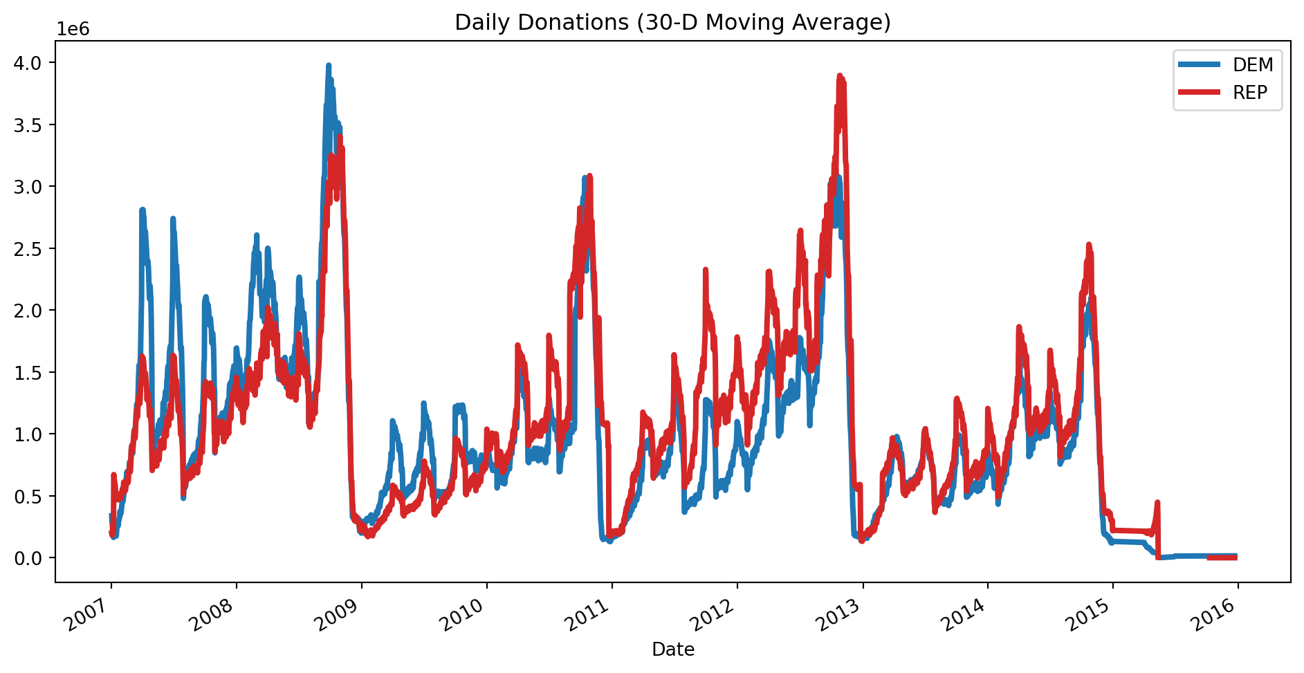

ax = (
    party_donations_dd
    .unstack("CMTE_PTY_AFFILIATION")
    .iloc[1:]
    .rolling("30D")
    .mean()
    [["DEM", "REP"]]
    .plot(color=["C0", "C3"], figsize=(12, 6), linewidth=3)
)
ax.set(title="Daily Donations (30-D Moving Average)", xlabel="Date")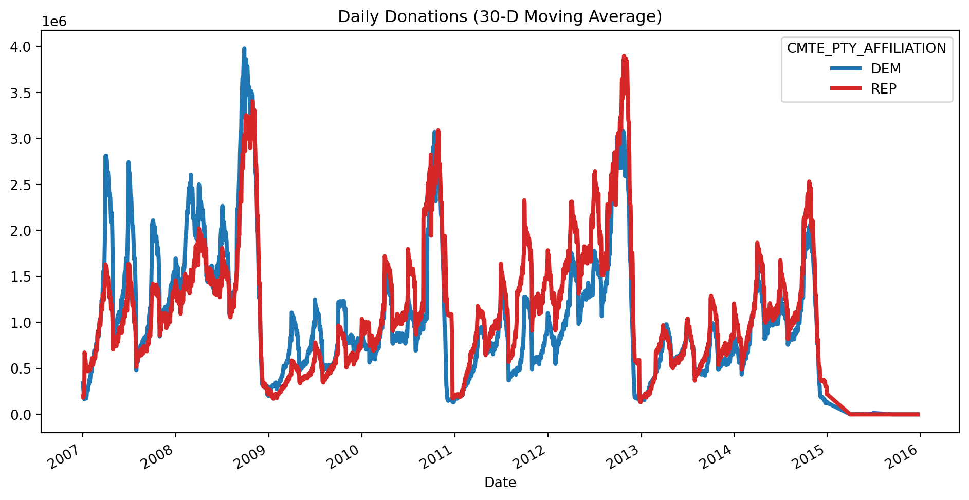

6.7 Polars vs PySpark

The Polars team released a benchmark comparing Polars to PySpark in June 2026, looking at single node and distributed performance on AWS. In the single node benchmark Polars was ~6.4x faster than PySpark, ranging from 3x to 38x faster per query. In the distributed benchmark Polars was ~3.2x faster than PySpark, ranging from 1.6x to 7.7x faster per query.