from pathlib import Path
from io import StringIO
from datetime import datetime, date
import requests
import polars as pl
import pandas as pd
import matplotlib.pyplot as plt

pl.Config.set_tbl_rows(5)
pd.options.display.max_rows = 5
data_path = Path("../data/ohlcv.pq")


def epoch_ms(dt: datetime) -> int:
    return int(dt.timestamp()) * 1000


if data_path.exists():
    ohlcv_pl = pl.read_parquet(data_path).set_sorted("time")

else:
    start = epoch_ms(datetime(2021, 1, 1))
    end = epoch_ms(datetime(2022, 1, 1))
    url = (
        "https://api.binance.com/api/v3/klines?symbol=BTCUSDT&"
        f"interval=1d&startTime={start}&endTime={end}"
    )
    resp = requests.get(url)
    time_col = "time"
    ohlcv_cols = [
        "open",
        "high",
        "low",
        "close",
        "volume",
    ]
    cols_to_use = [time_col, *ohlcv_cols]
    cols = cols_to_use + [f"ignore_{i}" for i in range(6)]
    ohlcv_pl = pl.from_records(resp.json(), orient="row", schema=cols).select(
        [
            pl.col(time_col).cast(pl.Datetime).dt.with_time_unit("ms").cast(pl.Date),
            pl.col(ohlcv_cols).cast(pl.Float64),
        ]
    ).set_sorted("time")
    ohlcv_pl.write_parquet(data_path)

ohlcv_pd = ohlcv_pl.with_columns(pl.col("time").cast(pl.Datetime)).to_pandas().set_index("time")5 Timeseries
Temporal data is an area in which Pandas actually far outshines R’s dataframe libraries. Things like resampling and rolling calculations are baked into the dataframe library and work quite well. Fortunately this is also true of Polars!
5.1 Get the data
We’ll download a year’s worth of daily price and volume data for Bitcoin:
5.2 Filtering
Pandas has special methods for filtering data with a DatetimeIndex. Since Polars doesn’t have an index, we just use .filter. I will admit the Pandas code is more convenient for things like filtering for a specific month:
ohlcv_pl.filter(
    pl.col("time").is_between(
        date(2021, 2, 1),
        date(2021, 3, 1),
        closed="left"
    )
)
shape: (28, 6)
| time | open | high | low | close | volume |
|---|---|---|---|---|---|
| date | f64 | f64 | f64 | f64 | f64 |
| 2021-02-01 | 33092.97 | 34717.27 | 32296.16 | 33526.37 | 82718.276882 |
| 2021-02-02 | 33517.09 | 35984.33 | 33418.0 | 35466.24 | 78056.65988 |
| 2021-02-03 | 35472.71 | 37662.63 | 35362.38 | 37618.87 | 80784.333663 |
| … | … | … | … | … | … |
| 2021-02-27 | 46276.88 | 48394.0 | 45000.0 | 46106.43 | 66060.834292 |
| 2021-02-28 | 46103.67 | 46638.46 | 43000.0 | 45135.66 | 83055.369042 |
ohlcv_pd.loc["2021-02"]| open | high | low | close | volume | |
|---|---|---|---|---|---|
| time | |||||
| 2021-02-01 | 33092.97 | 34717.27 | 32296.16 | 33526.37 | 82718.276882 |
| 2021-02-02 | 33517.09 | 35984.33 | 33418.00 | 35466.24 | 78056.659880 |
| ... | ... | ... | ... | ... | ... |
| 2021-02-27 | 46276.88 | 48394.00 | 45000.00 | 46106.43 | 66060.834292 |
| 2021-02-28 | 46103.67 | 46638.46 | 43000.00 | 45135.66 | 83055.369042 |
28 rows × 5 columns
5.3 Resampling
Resampling is like a special case of group_by for a time column. You can of course use regular .group_by with a time column, but it won’t be as powerful because it doesn’t understand time like resampling methods do.
There are two kinds of resampling: downsampling and upsampling.
5.3.1 Downsampling
Downsampling moves from a higher time frequency to a lower time frequency. This requires some aggregation or subsetting, since we’re reducing the number of rows in our data.
In Polars we use the .group_by_dynamic method for downsampling (we also use group_by_dynamic when we want to combine resampling with regular group_by logic).
(
    ohlcv_pl
    .group_by_dynamic("time", every="5d")
    .agg(pl.col(pl.Float64).mean())
)
shape: (74, 6)
| time | open | high | low | close | volume |
|---|---|---|---|---|---|
| date | f64 | f64 | f64 | f64 | f64 |
| 2020-12-29 | 29127.665 | 31450.0 | 28785.55 | 30755.01 | 92088.399186 |
| 2021-01-03 | 33577.028 | 36008.464 | 31916.198 | 35027.986 | 127574.470245 |
| 2021-01-08 | 38733.61 | 39914.548 | 34656.422 | 37655.352 | 143777.954392 |
| … | … | … | … | … | … |
| 2021-12-24 | 50707.08 | 51407.656 | 49540.152 | 50048.066 | 29607.160572 |
| 2021-12-29 | 46836.5525 | 48135.4925 | 45970.84 | 46881.2775 | 31098.406725 |
ohlcv_pd.resample("5d").mean()/tmp/ipykernel_3400377/1978683501.py:1: Pandas4Warning: 'd' is deprecated and will be removed in a future version, please use 'D' instead.
ohlcv_pd.resample("5d").mean()| open | high | low | close | volume | |
|---|---|---|---|---|---|
| time | |||||
| 2021-01-01 | 31084.316 | 33127.622 | 29512.818 | 32089.662 | 112416.849570 |
| 2021-01-06 | 38165.310 | 40396.842 | 35983.822 | 39004.538 | 118750.076685 |
| ... | ... | ... | ... | ... | ... |
| 2021-12-27 | 48521.240 | 49475.878 | 47087.400 | 47609.528 | 35886.943710 |
| 2022-01-01 | 46216.930 | 47954.630 | 46208.370 | 47722.650 | 19604.463250 |
74 rows × 5 columns
Resampling and performing multiple aggregations to each column:
(
    ohlcv_pl
    .group_by_dynamic("time", every="1w", start_by="friday")
    .agg([
        pl.col(pl.Float64).mean().name.suffix("_mean"),
        pl.col(pl.Float64).sum().name.suffix("_sum")
    ])
)
shape: (53, 11)
| time | open_mean | high_mean | low_mean | close_mean | volume_mean | open_sum | high_sum | low_sum | close_sum | volume_sum |
|---|---|---|---|---|---|---|---|---|---|---|
| date | f64 | f64 | f64 | f64 | f64 | f64 | f64 | f64 | f64 | f64 |
| 2021-01-01 | 32305.781429 | 34706.045714 | 31021.727143 | 33807.135714 | 117435.5928 | 226140.47 | 242942.32 | 217152.09 | 236649.95 | 822049.149598 |
| 2021-01-08 | 37869.797143 | 39646.105714 | 34623.334286 | 37827.52 | 135188.296617 | 265088.58 | 277522.74 | 242363.34 | 264792.64 | 946318.076319 |
| 2021-01-15 | 36527.891429 | 37412.2 | 33961.551429 | 35343.847143 | 94212.715129 | 255695.24 | 261885.4 | 237730.86 | 247406.93 | 659489.005903 |
| … | … | … | … | … | … | … | … | … | … | … |
| 2021-12-24 | 49649.114286 | 50439.622857 | 48528.25 | 49117.98 | 31126.709793 | 347543.8 | 353077.36 | 339697.75 | 343825.86 | 217886.96855 |
| 2021-12-31 | 46668.905 | 48251.445 | 45943.185 | 46969.79 | 27271.230605 | 93337.81 | 96502.89 | 91886.37 | 93939.58 | 54542.46121 |
ohlcv_pd.resample("W-Fri", closed="left", label="left").agg(['mean', 'sum'])/tmp/ipykernel_3400377/3740097180.py:1: Pandas4Warning: 'W-Fri' is deprecated and will be removed in a future version, please use 'W-FRI' instead.
ohlcv_pd.resample("W-Fri", closed="left", label="left").agg(['mean', 'sum'])| open | high | low | close | volume | ||||||
|---|---|---|---|---|---|---|---|---|---|---|
| mean | sum | mean | sum | mean | sum | mean | sum | mean | sum | |
| time | ||||||||||
| 2021-01-01 | 32305.781429 | 226140.47 | 34706.045714 | 242942.32 | 31021.727143 | 217152.09 | 33807.135714 | 236649.95 | 117435.592800 | 822049.149598 |
| 2021-01-08 | 37869.797143 | 265088.58 | 39646.105714 | 277522.74 | 34623.334286 | 242363.34 | 37827.520000 | 264792.64 | 135188.296617 | 946318.076319 |
| ... | ... | ... | ... | ... | ... | ... | ... | ... | ... | ... |
| 2021-12-24 | 49649.114286 | 347543.80 | 50439.622857 | 353077.36 | 48528.250000 | 339697.75 | 49117.980000 | 343825.86 | 31126.709793 | 217886.968550 |
| 2021-12-31 | 46668.905000 | 93337.81 | 48251.445000 | 96502.89 | 45943.185000 | 91886.37 | 46969.790000 | 93939.58 | 27271.230605 | 54542.461210 |
53 rows × 10 columns
5.3.2 Upsampling
Upsampling moves in the opposite direction, from low-frequency data to high frequency data. Since we can’t create new data by magic, upsampling defaults to filling the new rows with nulls (which we could then interpolate, perhaps). In Polars we have a special upsample method for this, while Pandas reuses its resample method.
ohlcv_pl.upsample("time", every="6h")
shape: (1_461, 6)
| time | open | high | low | close | volume |
|---|---|---|---|---|---|
| date | f64 | f64 | f64 | f64 | f64 |
| 2021-01-01 | 28923.63 | 29600.0 | 28624.57 | 29331.69 | 54182.925011 |
| 2021-01-01 | null | null | null | null | null |
| 2021-01-01 | null | null | null | null | null |
| … | … | … | … | … | … |
| 2021-12-31 | null | null | null | null | null |
| 2022-01-01 | 46216.93 | 47954.63 | 46208.37 | 47722.65 | 19604.46325 |
ohlcv_pd.resample("6h").mean()| open | high | low | close | volume | |
|---|---|---|---|---|---|
| time | |||||
| 2021-01-01 00:00:00 | 28923.63 | 29600.00 | 28624.57 | 29331.69 | 54182.925011 |
| 2021-01-01 06:00:00 | NaN | NaN | NaN | NaN | NaN |
| ... | ... | ... | ... | ... | ... |
| 2021-12-31 18:00:00 | NaN | NaN | NaN | NaN | NaN |
| 2022-01-01 00:00:00 | 46216.93 | 47954.63 | 46208.37 | 47722.65 | 19604.463250 |
1461 rows × 5 columns
5.4 Rolling / Expanding / EW
Polars supports all three of these, but they’re missing some of the methods that Pandas has. Custom rolling and expanding aggregations are supported in Polars using expr.rolling_map and expr.cumulative_eval respectively, but the docs recommend against using them for performance reasons.
close = pl.col("close")
ohlcv_pl.select(
    [
        pl.col("time"),
        close.alias("Raw"),
        close.rolling_mean(28).alias("28D MA"),
        (close.cum_sum() / close.cum_count()).alias("Expanding Average"),
        close.ewm_mean(alpha=0.03).alias("EWMA($\\alpha=.03$)"),
    ]
).to_pandas().set_index("time").plot()

plt.ylabel("Close ($)")
Text(0, 0.5, 'Close ($)')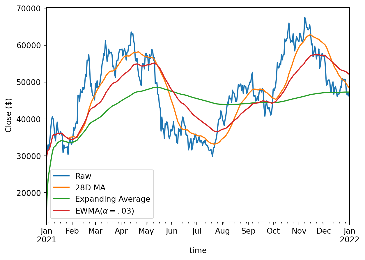
ohlcv_pd["close"].plot(label="Raw")
ohlcv_pd["close"].rolling(28).mean().plot(label="28D MA")
ohlcv_pd["close"].expanding().mean().plot(label="Expanding Average")
ohlcv_pd["close"].ewm(alpha=0.03).mean().plot(label="EWMA($\\alpha=.03$)")

plt.legend(bbox_to_anchor=(0.63, 0.27))
plt.ylabel("Close ($)")
Text(0, 0.5, 'Close ($)')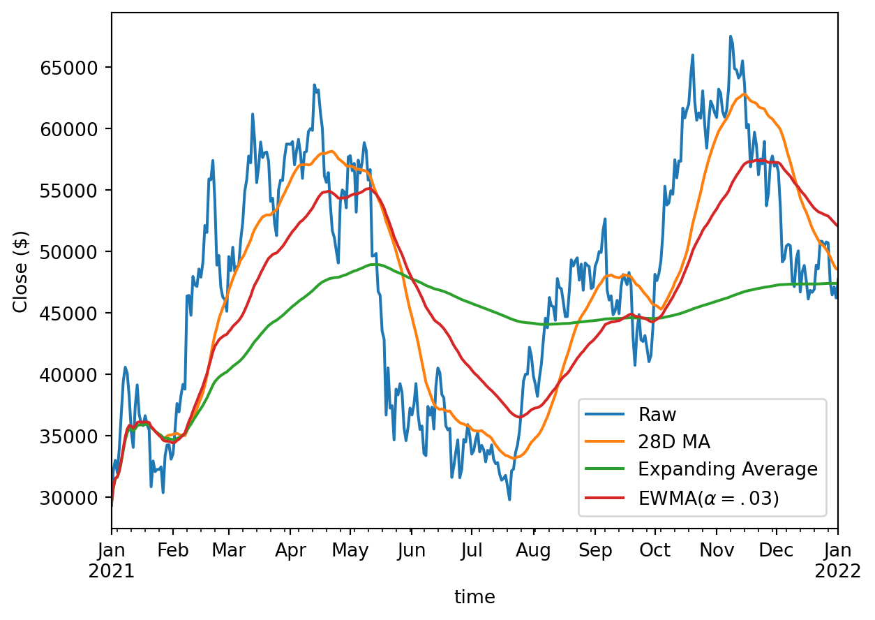
Polars doesn’t have an expanding_mean or cum_mean yet so we make do by combining cum_sum and cum_count. You could also use cumulative_eval, but it’s much slower on large columns, and the docs recommend against it for performance reasons.
5.4.1 Combining rolling aggregations
mean_std_pl = ohlcv_pl.select(
    [
        "time",
        pl.col("close").rolling_mean(30, center=True).alias("mean"),
        pl.col("close").rolling_std(30, center=True).alias("std"),
    ]
)
ax = mean_std_pl.to_pandas().set_index("time")["mean"].plot()
ax.fill_between(
    mean_std_pl["time"].to_numpy(),
    mean_std_pl["mean"] - mean_std_pl["std"],
    mean_std_pl["mean"] + mean_std_pl["std"],
    alpha=0.25,
)
plt.tight_layout()
plt.ylabel("Close ($)")
Text(29.33333333333334, 0.5, 'Close ($)')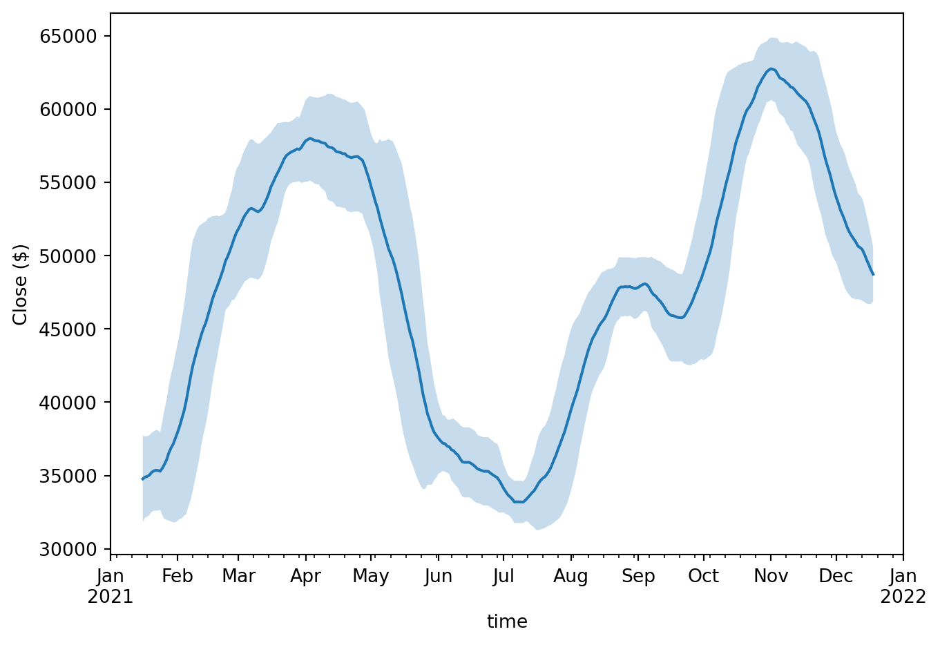
roll_pd = ohlcv_pd["close"].rolling(30, center=True)
mean_std_pd = roll_pd.agg(["mean", "std"])
ax = mean_std_pd["mean"].plot()
ax.fill_between(
    mean_std_pd.index,
    mean_std_pd["mean"] - mean_std_pd["std"],
    mean_std_pd["mean"] + mean_std_pd["std"],
    alpha=0.25,
)
plt.tight_layout()
plt.ylabel("Close ($)")
Text(29.33333333333334, 0.5, 'Close ($)')
5.5 Grab Bag
5.5.1 Offsets
Pandas has two similar objects for datetime arithmetic: DateOffset which respects calendar arithmetic, and Timedelta which respects absolute time arithmetic. DateOffset understands things like daylight savings time, and can work with holidays too.
Polars just has a Duration type which is like Pandas Timedelta.
ohlcv_pl.select(pl.col("time") + pl.duration(days=80))
shape: (366, 1)
| time |
|---|
| date |
| 2021-03-22 |
| 2021-03-23 |
| 2021-03-24 |
| … |
| 2022-03-21 |
| 2022-03-22 |
ohlcv_pd.index + pd.Timedelta(80, "D")DatetimeIndex(['2021-03-22', '2021-03-23', '2021-03-24', '2021-03-25',
'2021-03-26', '2021-03-27', '2021-03-28', '2021-03-29',
'2021-03-30', '2021-03-31',
...
'2022-03-13', '2022-03-14', '2022-03-15', '2022-03-16',
'2022-03-17', '2022-03-18', '2022-03-19', '2022-03-20',
'2022-03-21', '2022-03-22'],
dtype='datetime64[us]', name='time', length=366, freq=None)ohlcv_pd.index + pd.DateOffset(months=3, days=-10)DatetimeIndex(['2021-03-22', '2021-03-23', '2021-03-24', '2021-03-25',
'2021-03-26', '2021-03-27', '2021-03-28', '2021-03-29',
'2021-03-30', '2021-03-31',
...
'2022-03-13', '2022-03-14', '2022-03-15', '2022-03-16',
'2022-03-17', '2022-03-18', '2022-03-19', '2022-03-20',
'2022-03-21', '2022-03-22'],
dtype='datetime64[us]', name='time', length=366, freq=None)5.5.2 Holiday calendars
Not many people know this, but Pandas can do some quite powerful stuff with Holiday Calendars. Some, but not all, of this functionality is available in Polars in the expr.dt namespace.
5.5.3 Timezones
Suppose we know that our timestamps are UTC, and we want to see what time it was in US/Eastern:
(
    ohlcv_pl
    .with_columns(
        pl.col("time")
        .cast(pl.Datetime)
        .dt.replace_time_zone("UTC")
        .dt.convert_time_zone("US/Eastern")
    )
)
shape: (366, 6)
| time | open | high | low | close | volume |
|---|---|---|---|---|---|
| datetime[μs, US/Eastern] | f64 | f64 | f64 | f64 | f64 |
| 2020-12-31 19:00:00 EST | 28923.63 | 29600.0 | 28624.57 | 29331.69 | 54182.925011 |
| 2021-01-01 19:00:00 EST | 29331.7 | 33300.0 | 28946.53 | 32178.33 | 129993.873362 |
| 2021-01-02 19:00:00 EST | 32176.45 | 34778.11 | 31962.99 | 33000.05 | 120957.56675 |
| … | … | … | … | … | … |
| 2021-12-30 19:00:00 EST | 47120.88 | 48548.26 | 45678.0 | 46216.93 | 34937.99796 |
| 2021-12-31 19:00:00 EST | 46216.93 | 47954.63 | 46208.37 | 47722.65 | 19604.46325 |
(
    ohlcv_pd
    .tz_localize('UTC')
    .tz_convert('US/Eastern')
)| open | high | low | close | volume | |
|---|---|---|---|---|---|
| time | |||||
| 2020-12-31 19:00:00-05:00 | 28923.63 | 29600.00 | 28624.57 | 29331.69 | 54182.925011 |
| 2021-01-01 19:00:00-05:00 | 29331.70 | 33300.00 | 28946.53 | 32178.33 | 129993.873362 |
| ... | ... | ... | ... | ... | ... |
| 2021-12-30 19:00:00-05:00 | 47120.88 | 48548.26 | 45678.00 | 46216.93 | 34937.997960 |
| 2021-12-31 19:00:00-05:00 | 46216.93 | 47954.63 | 46208.37 | 47722.65 | 19604.463250 |
366 rows × 5 columns
5.6 Conclusion
Polars has really good time series support, though expanding aggregations and holiday calendars are niches in which it is somewhat lacking. Pandas DateTimeIndexes are quite cool too, even if they do bring some pain.